Synchronisation and the Kuramoto Model
Collective behaviour, phase transitions, and network topology in coupled oscillator systems
1. Introduction
Recently, I was cleaning up some of my old folders and found a notebook I had written a few years ago on the Kuramoto model for a course on complex systems. I had been fascinated by the generality of the synchronisation phenomenon, and I had wanted to understand it a bit better and share that understanding with others. Back then my numerical coding skills were very minimal and the notebook was a bit rough around the edges, but it contained a complete derivation of the main results and some numerical simulations. I decided to polish the assignment and turn it into an article that could be read independently of the code, but also clean up the code with the help of LLMs, as they became very good at generating or cleaning code. Together with this article,I posted the rendered notebook here.
Synchronisation is one of nature's most pervasive collective phenomena. Fireflies in South-East Asia flash in near-perfect unison. Neurons in the brain lock into coherent rhythms during cognition and sleep. Pacemaker cells in the heart coordinate their firing to sustain a steady beat. Arrays of superconducting Josephson junctions spontaneously phase-lock when coupled. Power-grid generators must maintain synchronicity to deliver alternating current at a stable frequency. In each of these settings, a large population of individually oscillating units, each with its own intrinsic rhythm, manages, under sufficient coupling, to surrender some of its individuality and beat together.
Like many good models, the Kuramoto model captures the essence of a complex phenomenon (in this case synchronisation) with a minimal set of assumptions. That is, it describes a population of oscillators that, before coupling, are independent of one another. Their natural frequencies $\omega_i$ are randomly distributed, and the coupling then tries to align their phases. In such a setup, only phase differences matter, the interaction is periodic and it is zero when the phases are equal. The model is analytically tractable, and it exhibits a genuine phase transition in the limit of large number of oscillators $N$.
In this post I go through the parts of the model that I find most useful: the equations of motion, the order parameter, the self-consistency argument that gives a critical coupling strength $K_c$, and the numerical experiments that make the transition visible. Towards the end, I also include the Watts-Strogatz network extension, as I thought it fitting in the context social networks or neural networks, among others.
2. The Kuramoto Model
Let me start by introducing the model through its equations of motion. Each oscillator is described only by a phase angle $\theta_i(t) \in [0, 2\pi)$. Without coupling, the oscillators are independent and each simply rotates at its own natural frequency, $\dot\theta_i = \omega_i$, with the $\omega_i$ sampled from $g(\omega)$. Coupling then adds a correction that depends on whether the other oscillators are ahead of it or behind it:
Here $K \geq 0$ controls how strongly the oscillators try to pull one another into step. The factor $1/N$ keeps the total coupling from blowing up as the population grows, and the sine is the simplest periodic coupling that makes nearby phases attract.
One of the first useful checks is that the coupling does not change the average rotation rate. Let the mean frequency $\bar\omega = \frac{1}{N}\sum_{i=1}^N \omega_i$.
If we sum the equations of motion over all oscillators, the coupling term cancels pair by pair because $\sin(\theta_j - \theta_i) = -\sin(\theta_i - \theta_j)$:
This means that the coupling can redistribute phase velocities inside the population, but it cannot accelerate or decelerate the average oscillator. When a synchronized group forms, it rotates at this mean frequency.
It is cleaner to remove this overall rotation and work in a frame co-moving with the mean frequency. Let us define $\phi_i(t) = \theta_i(t) - \bar\omega\, t$, which gives
Without loss of generality one can take $g(\omega)$ to be centred at zero (i.e. $\bar\omega = 0$), so that the natural frequencies in the rotating frame are $\Delta_i = \omega_i - \bar\omega$ with $\sum_i \Delta_i = 0$.
3. Moving Towards Minima of a Potential Landscape
3.1 The Lyapunov functional
There is a useful way of reading the rotating-frame dynamics as motion down a landscape. In dynamical-systems language, the object that defines this landscape is a Lyapunov functional $\mathcal{H}(\boldsymbol\phi)$: it is not a conserved energy, but a quantity that decreases as the phases evolve.
Let the frequency mismatch be defined as $\Delta_i=\omega_i-\bar\omega$. Then we can introduce the Lyapunov functional
The first term rewards phase alignment. The second term represents the fact that each oscillator has its own preferred natural frequency. In this language, synchronization is the result of the alignment term becoming strong enough to overcome the frequency disorder.
The reason this functional is useful is that it generates the Kuramoto dynamics as a gradient flow:
Therefore
This is the precise sense in which the rotating-frame Kuramoto dynamics move towards minima of a landscape. The phases "flow" downhill until the rotating-frame velocities vanish. Many initial phase configurations can therefore end up at the same locked state, which is the behavior of an attracting dissipative system.
3.2 The magnetic analogy
As a condensed matter physicist, the first term immediately looks familiar:
If $\phi_i$ is read as an XY spin angle, this is exactly the form of a mean-field ferromagnetic exchange energy. It wants all the angles to align. This is why the Kuramoto model often feels close to a magnetic ordering problem: synchronization and ferromagnetism both involve an alignment tendency competing against something that disrupts order.
But the analogy stops right there. In the Kuramoto problem, $\mathcal{H}$ is a Lyapunov functional for first-order dissipative phase dynamics. It must decrease along the trajectories. In an equilibrium magnet, a Hamiltonian is an energy functional used to define statistical weights, and in Hamiltonian mechanics it would generate conservative motion. Those are different conditions on the same-looking mathematical object.
3.3 Equilibrium conditions and the synchronized state
Stationary phase configurations are obtained by setting the rotating-frame velocities (2) to zero. This gives the balance condition
It is useful to pause on the simplest case, where all natural frequencies are equal ($\omega_i=\bar\omega$ for all $i$). Then the right-hand side vanishes, and the most natural stable solution is the fully synchronized one, $\phi_i=\phi^*$ for all $i$. If there is no frequency disorder, all oscillators can simply choose the same phase in the rotating frame.
Once the frequencies are different, perfect equality of all phases is no longer generally possible. The interesting question is then how much coupling is needed before a coherent locked group appears.
4. The Order Parameter and the Phase Transition
4.1 The order parameter
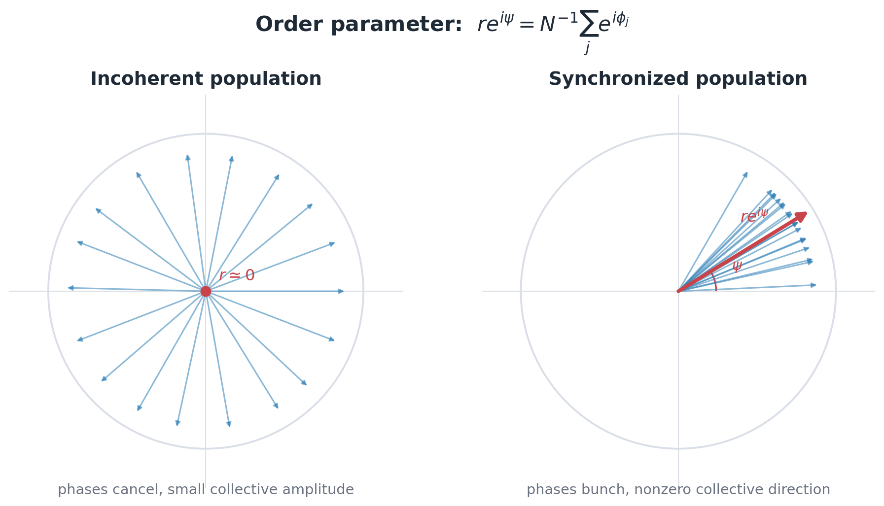
The order parameter is the object that makes the transition to synchronization visible. It packages the whole population into one complex number:
Here $r(t) \in [0,1]$ measures coherence. If the phases are spread uniformly around the circle, their complex phases cancel and $r \approx 0$. If all phases coincide, they add constructively and $r = 1$. The angle $\psi(t)$ is the average phase direction.
This order parameter in fact simplifies the description of the dynamics. Multiplying both sides of (5) by $e^{-i\phi_i}$ and taking the imaginary part shows that $\frac{K}{N}\sum_j \sin(\phi_j - \phi_i) = Kr\sin(\psi - \phi_i)$. The equations of motion then reduce to
Each oscillator now sees only the collective mean field $(r,\psi)$, not the individual phases of all its partners. The all-to-all interaction has collapsed into one scalar amplitude and one collective angle.
At a locked configuration, the rotating-frame velocity vanishes. Equation (6) then gives the balance between the oscillator's frequency mismatch and the pull of the collective field:
This compact relation is the picture to keep in mind: oscillators close enough to the collective frequency can sit at a fixed phase offset, while oscillators too far away keep drifting.
4.2 Self-consistency and the critical coupling
The critical coupling comes from separating the population into two intuitive groups. In a large system with a smooth frequency distribution $g(\omega)$, a stationary mean field can hold some oscillators in place, while the rest continue to drift. Each oscillator then either:
- Phase-locks (frequency-entrained) to the mean field if $|\omega_i - \bar\omega| \leq Kr$. From (7), its locked phase satisfies $\phi_i - \psi = \arcsin\!\left(\frac{\omega_i - \bar\omega}{Kr}\right)$.
- Drifts if $|\omega_i - \bar\omega| > Kr$. These oscillators rotate at their own speed and, averaged over time, make no net contribution to the order parameter by symmetry of $g$.
The order parameter has to be self-consistent: the value of $r$ that creates the locked group must also be the value produced by that locked group. Each locked oscillator contributes $\cos(\phi_i-\psi)$ to the real part of the order parameter. In the continuum limit this gives
For the synchronized branch, $r>0$, so dividing by $r$ gives the self-consistency equation:
This equation is the compact version of the transition. Below a certain coupling it has no positive solution. Above it, a nonzero coherent branch appears.
Near the onset of synchronization, $r$ is very small. Then $g(Kr\sin\vartheta)$ can be replaced by its value at the center of the distribution, $g(0)$, and the remaining integral is just $\int_{-\pi/2}^{\pi/2}\cos^2\vartheta\,d\vartheta=\pi/2$. This gives
This is the result I find most satisfying in the model. The critical coupling depends only on the height of the frequency distribution at its peak. A broader distribution has smaller $g(0)$, so the oscillators are harder to lock and the required coupling increases. In the examples below, this is why the broader Gaussian case needs a larger coupling than the narrower uniform distribution.
4.3 Symmetry breaking and the zero mode
Another way to understand the transition is to look at the long-time state selected by the dynamics for each value of $K$. After transients have died out, the system has reached a stable or statistically stationary state in the rotating frame. That long-time state can still be disordered, or it can be synchronized.
The symmetry behind the discussion is the global phase rotation
Strictly speaking, this continuous symmetry is a $U(1)$ symmetry, or equivalently the rotation group $SO(2)$. One sometimes loosely says "$O(2)$" when thinking about XY spins, but $O(2)$ also contains reflections, $\phi_i\to-\phi_i+\Theta$. The zero-mode discussion below only needs the continuous rotation part.
The equations do not care where the origin of phase is chosen. Equivalently, the order parameter transforms as
For $K<K_c$, the incoherent state has $r=0$ in the infinite-size limit. The phases are spread around the circle, so there is no meaningful collective angle $\psi$. Rotating the whole population changes nothing macroscopically. The long-time state respects the rotational symmetry.
For $K>K_c$, the situation changes. The order parameter has a nonzero magnitude, $r>0$, and therefore points in some direction $\psi$. The equations are still rotationally symmetric: if one synchronized state with phase $\psi$ is possible, then every rotated state with phase $\psi+\Theta$ is equally possible. But a particular run of the dynamics selects one of them, usually through the initial condition. This is the symmetry-breaking picture: the equations have the symmetry, while the synchronized long-time state chooses a direction.
The same rotational symmetry also has a concrete stability signature. If all phases are shifted by the same constant, $\phi_i \to \phi_i + \Theta$, nothing physical changes. In other words, $\mathcal{H}$ does not care where we place the overall phase origin. To make this more concrete, one can look at the Jacobian matrix of the dynamical system. The Jacobian is the linear stability matrix: it tells us how small perturbations of the phases grow, decay, or remain neutral near a locked state. If a perturbation feels no restoring force, it appears as a zero eigenvalue of this matrix. The rotational symmetry therefore has an important consequence for the Jacobian, whose elements are
This symmetry means that the uniform vector $\mathbf{1}=(1,1,\ldots,1)^T$ is a zero mode of the Jacobian. One can check it directly: the $i$-th component of $J\mathbf{1}$ is $\frac{K}{N}\sum_j \cos(\phi_j-\phi_i)-\frac{K}{N}\sum_k\cos(\phi_k-\phi_i)=0$. A collective shift of all phases therefore costs no restoring force.
This is the same kind of zero mode that appears whenever a continuous rotational symmetry is spontaneously broken. A compact way of phrasing the discussion I had while writing these notes is that $r$ plays the role of a magnetization-like amplitude, while $\psi$ is the chosen collective direction. Below $K_c$, there is no meaningful direction because $r=0$ in the $N\to\infty$ limit. Above $K_c$, the synchronized attractor fixes the shape of the phase pattern, but not its absolute angle: every rotated pattern is equivalent. Perturbations that change relative phases can relax, while the global shift $\psi\to\psi+\Theta$ is neutral. In that precise sense, the Jacobian zero mode is Goldstone-like, although in the all-to-all Kuramoto model it is a global phase mode rather than a spatial spin-wave mode.
This is also where the comparison with the XY magnet has to be handled carefully. The Kuramoto transition described here is a mean-field synchronization transition: the global order parameter $r$ becomes nonzero when a macroscopic set of oscillators locks to the collective frequency. This is close in spirit to mean-field magnetic ordering, where an exchange term favors a nonzero magnetization.
So the analogy is useful at the level of alignment and mean-field ordering, but the framework describes a different transition: collective frequency locking in a population of coupled oscillators. The most useful way for me to keep the analogy under control is to translate between the dynamical-systems and statistical-mechanics languages in the table below:
| Dynamical systems | Statistical mechanics |
|---|---|
| fixed point or locked attractor | free-energy extremum |
| Jacobian $J$ | Hessian of the free energy $H$ |
| stable if perturbations decay | stable if free energy increases under perturbations |
| zero eigenvalue of $J$ | zero-curvature direction of $F$ |
| neutral mode | flat direction / Goldstone mode |
5. Numerical Studies
5.1 Numerical method
In the notebook I integrate (1) using the explicit Euler method with time step $\Delta t$. The useful computational trick is to exploit the order parameter directly: once $r(t)$ and $\psi(t)$ are computed from the complex average $\frac{1}{N}\sum_j e^{i\theta_j}$, the update step for all $N$ oscillators reduces to a single vectorised operation, $$\theta_i^{(t+\Delta t)} = \theta_i^{(t)} + \Delta t\!\left(\omega_i + K\,r^{(t)}\sin\!\bigl(\psi^{(t)} - \theta_i^{(t)}\bigr)\right),$$ which requires no pairwise sums and runs efficiently with NumPy broadcasting. Initial phases $\theta_i(0)$ are drawn uniformly from $[0, 2\pi)$.
5.2 Two dynamical regimes
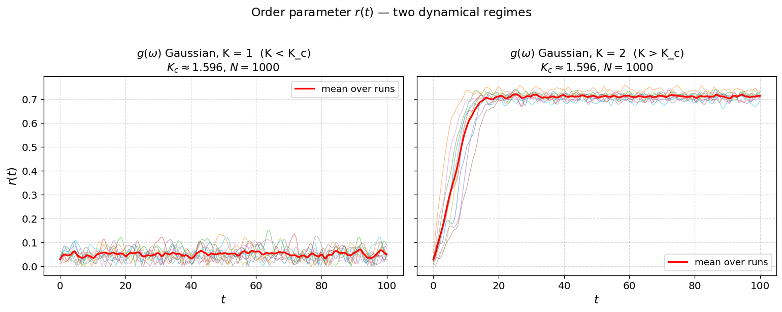
A simple comparison already shows the transition. I simulated $N=1000$ oscillators with Gaussian frequencies over $t \in [0,100]$ at two couplings: $K=1<K_c$ and $K=2>K_c$. Below $K_c$, the order parameter stays close to zero and the oscillators remain incoherent. Above $K_c$, $r(t)$ grows from its initially small value and settles near $r_\infty\approx0.72$, signalling a macroscopic synchronized fraction.
5.3 Effect of initial conditions: fixed $\omega$ versus fixed $\boldsymbol\theta(0)$
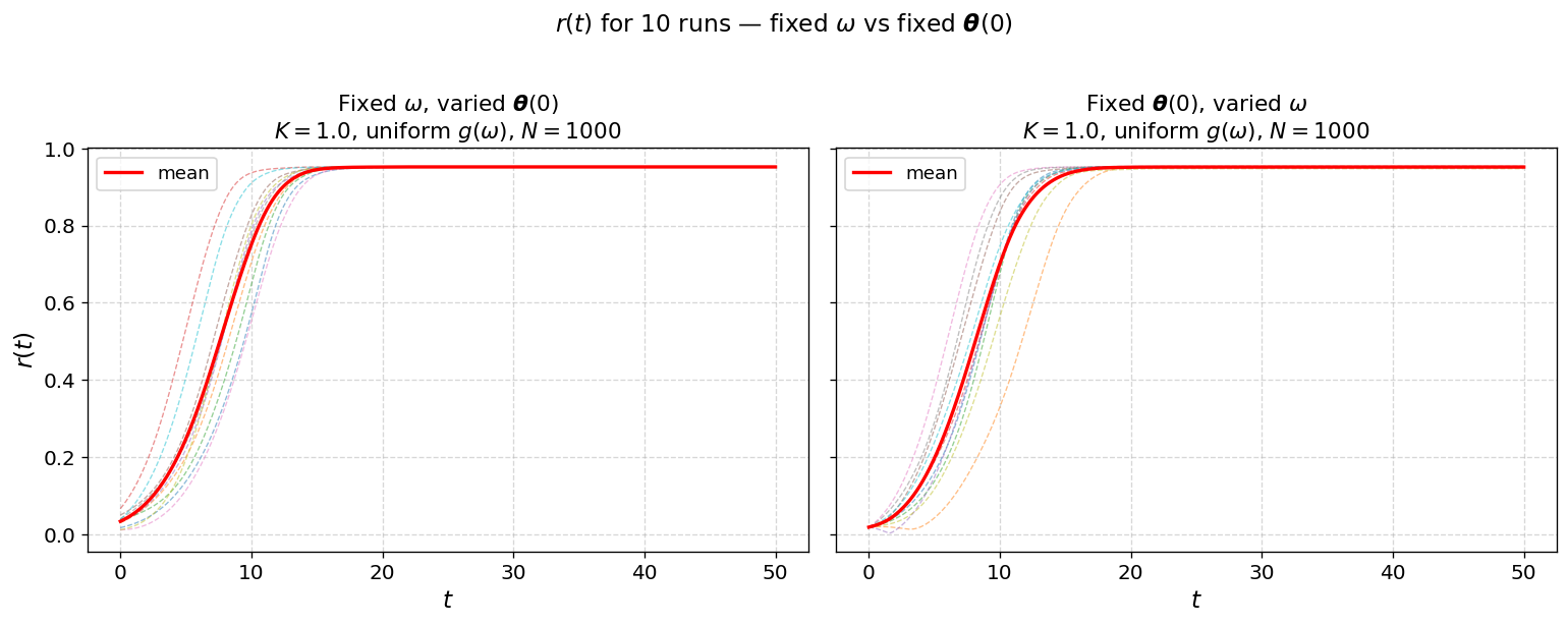
I also used the notebook to check how much the dynamics depend on the random choices made at the start. For $K=1$ with uniformly distributed frequencies, the system is already above $K_c=2/\pi$. If I keep the natural frequencies fixed and only resample the initial phases, the curves $r(t)$ vary less from run to run. If I keep the initial phases fixed and resample the frequencies, the spread is larger, because the particular draw of $\omega_i$ affects the transient dynamics more strongly. In these runs the standard deviation peaks at about $0.245$ for fixed $\boldsymbol\theta(0)$ and $0.173$ for fixed $\boldsymbol\omega$.
5.4 Steady-state coherence $r_\infty$ versus coupling $K$
The more satisfying numerical check is to scan $K$ and compare the steady-state value $r_\infty(K)$ with the self-consistency equation. I scan $K$ from $0$ to $5$, use finer sampling near the critical point, and average over 5 independent realizations. The agreement is excellent: the simulation follows the theoretical curve closely, with the largest scatter near $K_c$, exactly where finite-size fluctuations should matter most.
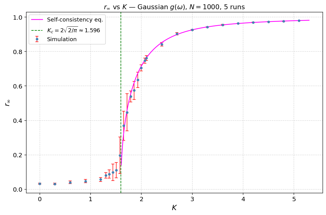
Extracting $K_c$ from the peak of the run-to-run standard deviation gives $K_c^{\rm sim}\approx1.65$ for the Gaussian case, compared with $K_c^{\rm theo}=2\sqrt{2/\pi}\approx1.596$. That is a deviation of about $3.4\%$, which is reasonable for a finite system. For the uniform distribution, the estimate is $K_c^{\rm sim}\approx0.64$, within $0.5\%$ of the theoretical value $2/\pi\approx0.637$.
6. Kuramoto on Watts–Strogatz Networks
6.1 Small-world topology
The old notebook also explored what happens when the all-to-all assumption is relaxed. That is important, because most physical networks are not fully connected. A simple way to interpolate between local and random connectivity is the Watts-Strogatz small-world network $\mathrm{WS}(N,2r,p)$ [2]. We start from a ring where each node talks to its nearby neighbours, then rewire each edge with probability $p$. As $p$ grows, the network moves from a local ring to a more random graph, passing through the small-world regime where a few long-range shortcuts dramatically shorten distances.
The useful point of the Watts-Strogatz construction is that it separates two network intuitions. At $p=0$ the graph is local and highly structured: nearby nodes share neighbours, but information has to travel around the ring. As $p$ increases, a small number of rewired edges creates shortcuts between distant parts of the graph. This can greatly reduce typical path lengths before the network looks completely random. I only use this construction here to ask how shortcuts affect synchronization thresholds; the network-theory side, including clustering and path lengths, belongs more naturally in the related planned post on complex networks and the Watts-Strogatz model.
On such a network the Kuramoto dynamics become
where $\mathcal{G}(i)$ is the set of neighbours of node $i$ after rewiring, and the coupling is normalised by the initial degree $2r$ so that the interaction strength per connection is comparable across networks.
6.2 The ring-lattice limit: $p = 0$
When $p=0$, no rewiring occurs and every oscillator talks only to its local neighbours. In that limit, no finite coupling synchronizes the full ring. The intuition is simple: local interactions alone do not carry phase information efficiently across the whole system. In the simulations, $r_\infty$ remains small even when the coupling is much larger than the mean-field $K_c$, consistent with the literature [3].
6.3 Effect of rewiring: $K_c$ as a function of $p$
As soon as a few long-range edges are added, the situation changes. Even a small rewiring probability can make global synchronization possible at finite $K$. In the notebook I estimate $K_c(p)$ as the value of $K$ where $r_\infty(K)$ crosses half its maximum. The resulting curve is well described by
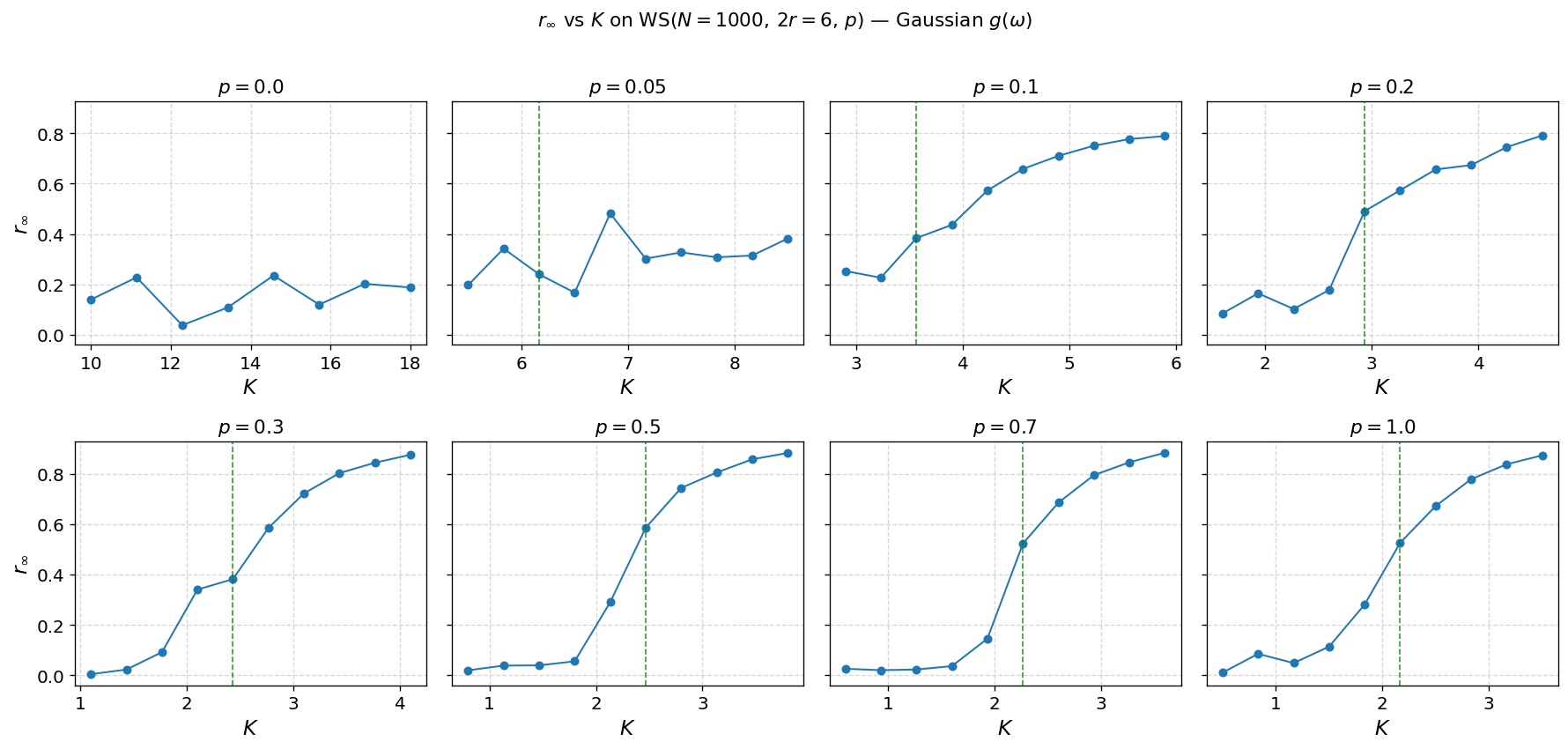
This is consistent with results reported in the literature [3]. The divergence as $p \to 0$ is the local-ring limit reappearing, while the constant offset is approached as the network becomes more random and more mean-field-like.
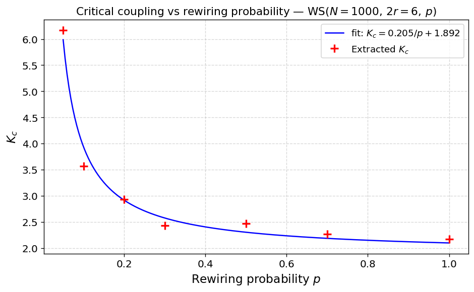
This is the part of the network story I find most intuitive. Long-range edges are shortcuts for phase information. They allow distant pieces of the ring to feel each other, so the system does not need enormous local coupling to coordinate. A small amount of randomness already changes the collective behavior dramatically.
7. Conclusion
What I enjoy about the Kuramoto model is that it gives a lot of physics for very little machinery. The critical coupling $K_c=2/(\pi g(0))$, the self-consistency equation for $r$, the downhill relaxation in a Lyapunov potential, and the neutral mode from rotational symmetry can all be seen with a few pages of algebra and a modest notebook.
The Watts-Strogatz extension is a useful reminder that topology is not decoration. It changes the threshold for collective behavior. Going from a local ring to a network with shortcuts is not a small technical modification; it changes whether global synchronization is possible at accessible coupling strengths.
This is also what makes the model feel contemporary to me. Many real networks are mostly local: people talk to colleagues, friends, neighbours, or nearby institutions. But globalization, online platforms, travel, and long-range collaborations add a small number of links between otherwise distant communities. The Watts-Strogatz picture says that such shortcuts can be disproportionately important. They do not need to replace local structure; a few long-range connections can already let information, rhythms, opinions, or conventions travel across the whole network much more efficiently. In that sense, synchronization is not just about stronger coupling. It is also about the architecture through which coupling is routed.
References
- Acebrón, J. A. et al. The Kuramoto model: A simple paradigm for synchronization phenomena. Reviews of Modern Physics 77, 137 (2005).
- Watts, D. J. & Strogatz, S. H. Collective dynamics of 'small-world' networks. Nature 393, 440–442 (1998).
- Hong, H., Choi, M. Y. & Kim, B. J. Synchronization on small-world networks. Physical Review E 65, 026139 (2002).